Linguagem R: Manipulação de Dados

Jose Storopoli

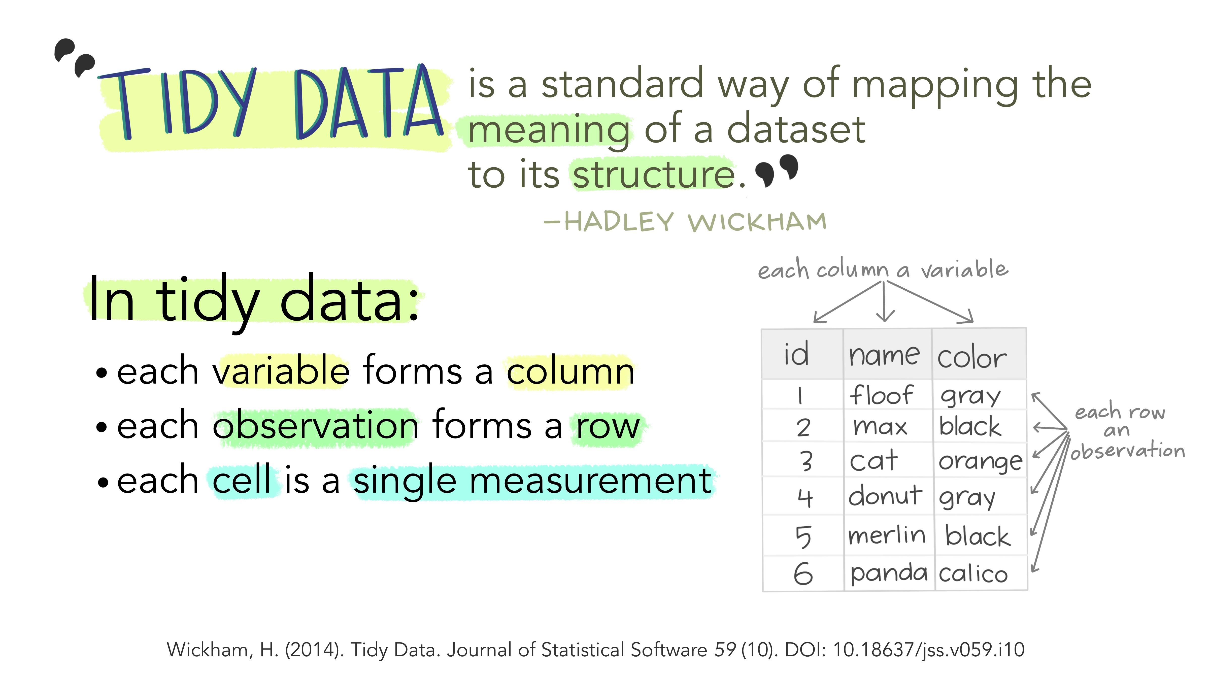
Figure 1: Tidy Data

O que é Tidy Data?

cada variável uma coluna
cada observação uma linha
cada célula uma mensuração única

O pipe `%>%`

x %>% f(y) vira f(x, y)

x %>% f(y) %>% f(z) vira f(f(x, y), z)

library(magrittr)

# atalho é CTRL + SHIFT + M

c(0:10, NA) %>%
  mean(na.rm = TRUE) %>% 
  print() %>% 
  message() %>% 
  message()

[1] 5

Como ler dados com o `{readr}`

Vamos começar com o primeiro passo da análise de dados: a importação dos dados.

Para isso o {tidyverse} possui um pacote chamado {readr}.

read_csv(): CSV padrão americano
read_csv2(): CSV padrão europeu/brasileiro
read_tsv(): TSV
read_delim(): Coringa

Na pasta datasets/ temos diversos datasets interessantes:

adult.csv
countries_of_the_world.csv
covid_19_data.csv: versão 147 de 27/02/2021.

Se vocês quiserem ler arquivos .xlsx ou .xls usem o pacote {readxl}

`col_types` – O argumento que eu mais uso em `read_*()`

library(readr)
adult <- read_csv("datasets/adult.csv",
                  col_types = "_iffifffif")

countries <- read_csv("datasets/countries_of_the_world.csv", 
    col_types = cols(Population = col_integer(), 
        `Net migration` = col_double()), 
    locale = locale(decimal_mark = ","))

covid <- read_csv("datasets/covid_19_data.csv", 
    col_types = cols(SNo = col_skip(), ObservationDate = col_date(format = "%m/%d/%Y")))

Manipulação de dados com o `{dplyr}`

Figure 2: dplyr

Selecionar Variáveis – `dplyr::select()`

library(dplyr)
adult_clean <- adult %>% 
  select(age, workclass, education,
         education_num = `educational-num`,
         marital_status = `marital-status`,
         race, gender,
         hours_per_week = `hours-per-week`,
         income)

OBS: Tem a função rename_with do {dplyr} versão 1.0.

adult %>% 
  rename_with(~gsub("-", "_", .x))

# A tibble: 48,842 × 9
     age workclass educa…¹ educa…² marit…³ race  gender hours…⁴ income
   <int> <fct>     <fct>     <int> <fct>   <fct> <fct>    <int> <fct> 
 1    25 Private   11th          7 Never-… Black Male        40 <=50K 
 2    38 Private   HS-grad       9 Marrie… White Male        50 <=50K 
 3    28 Local-gov Assoc-…      12 Marrie… White Male        40 >50K  
 4    44 Private   Some-c…      10 Marrie… Black Male        40 >50K  
 5    18 ?         Some-c…      10 Never-… White Female      30 <=50K 
 6    34 Private   10th          6 Never-… White Male        30 <=50K 
 7    29 ?         HS-grad       9 Never-… Black Male        40 <=50K 
 8    63 Self-emp… Prof-s…      15 Marrie… White Male        32 >50K  
 9    24 Private   Some-c…      10 Never-… White Female      40 <=50K 
10    55 Private   7th-8th       4 Marrie… White Male        10 <=50K 
# … with 48,832 more rows, and abbreviated variable names ¹education,
#   ²educational_num, ³marital_status, ⁴hours_per_week

adult %>% 
  rename_with(~gsub("-", "_", .x)) %>% 
  select(where(is.factor)) %>% 
  select(-workclass) %>% 
  rename_all(~paste0("antigo_", .x))

# A tibble: 48,842 × 5
   antigo_education antigo_marital_status antigo_race antigo…¹ antig…²
   <fct>            <fct>                 <fct>       <fct>    <fct>  
 1 11th             Never-married         Black       Male     <=50K  
 2 HS-grad          Married-civ-spouse    White       Male     <=50K  
 3 Assoc-acdm       Married-civ-spouse    White       Male     >50K   
 4 Some-college     Married-civ-spouse    Black       Male     >50K   
 5 Some-college     Never-married         White       Female   <=50K  
 6 10th             Never-married         White       Male     <=50K  
 7 HS-grad          Never-married         Black       Male     <=50K  
 8 Prof-school      Married-civ-spouse    White       Male     >50K   
 9 Some-college     Never-married         White       Female   <=50K  
10 7th-8th          Married-civ-spouse    White       Male     <=50K  
# … with 48,832 more rows, and abbreviated variable names
#   ¹antigo_gender, ²antigo_income

Professor eu gosto de camelCase e agora?

Não tema, tem o pacote {janitor}

library(janitor)
adult %>% clean_names(case = "lower_camel")

# A tibble: 48,842 × 9
     age workclass educa…¹ educa…² marit…³ race  gender hours…⁴ income
   <int> <fct>     <fct>     <int> <fct>   <fct> <fct>    <int> <fct> 
 1    25 Private   11th          7 Never-… Black Male        40 <=50K 
 2    38 Private   HS-grad       9 Marrie… White Male        50 <=50K 
 3    28 Local-gov Assoc-…      12 Marrie… White Male        40 >50K  
 4    44 Private   Some-c…      10 Marrie… Black Male        40 >50K  
 5    18 ?         Some-c…      10 Never-… White Female      30 <=50K 
 6    34 Private   10th          6 Never-… White Male        30 <=50K 
 7    29 ?         HS-grad       9 Never-… Black Male        40 <=50K 
 8    63 Self-emp… Prof-s…      15 Marrie… White Male        32 >50K  
 9    24 Private   Some-c…      10 Never-… White Female      40 <=50K 
10    55 Private   7th-8th       4 Marrie… White Male        10 <=50K 
# … with 48,832 more rows, and abbreviated variable names ¹education,
#   ²educationalNum, ³maritalStatus, ⁴hoursPerWeek

Ordenar variáveis com `dplyr::arrange()`

adult_clean %>% 
  arrange(-age, education_num) %>% 
  select(age, education_num)

# A tibble: 48,842 × 2
     age education_num
   <int>         <int>
 1    90             2
 2    90             4
 3    90             4
 4    90             4
 5    90             5
 6    90             6
 7    90             6
 8    90             7
 9    90             7
10    90             9
# … with 48,832 more rows

Frequencias com `dplyr::count()`

OBS: vamos ver muito essa função quando falarmos de group_by()

adult_clean %>% 
  count(age, income, sort = TRUE)

# A tibble: 142 × 3
     age income     n
   <int> <fct>  <int>
 1    23 <=50K   1307
 2    24 <=50K   1162
 3    22 <=50K   1161
 4    25 <=50K   1119
 5    27 <=50K   1117
 6    20 <=50K   1112
 7    28 <=50K   1101
 8    21 <=50K   1090
 9    26 <=50K   1068
10    19 <=50K   1050
# … with 132 more rows

Manipular Variáveis – `dplyr::mutate()`

Odeio potência de 10

use options(scipen = 999, digits = 2)

options(scipen = 999, digits = 2)
countries <- countries %>% clean_names()

countries %>% 
  mutate(
    log_pop = log(population),
    area_sq_km = area_sq_mi * 2.5899985,
    pop_density_per_sq_km = population / area_sq_km)

# A tibble: 227 × 23
   country      region popul…¹ area_…² pop_d…³ coast…⁴ net_m…⁵ infan…⁶
   <chr>        <chr>    <int>   <dbl>   <dbl>   <dbl>   <dbl>   <dbl>
 1 Afghanistan  ASIA …  3.11e7  647500    48      0      23.1   163.  
 2 Albania      EASTE…  3.58e6   28748   125.     1.26   -4.93   21.5 
 3 Algeria      NORTH…  3.29e7 2381740    13.8    0.04   -0.39   31   
 4 American Sa… OCEAN…  5.78e4     199   290.    58.3   -20.7     9.27
 5 Andorra      WESTE…  7.12e4     468   152.     0       6.6     4.05
 6 Angola       SUB-S…  1.21e7 1246700     9.7    0.13    0     191.  
 7 Anguilla     LATIN…  1.35e4     102   132.    59.8    10.8    21.0 
 8 Antigua & B… LATIN…  6.91e4     443   156     34.5    -6.15   19.5 
 9 Argentina    LATIN…  3.99e7 2766890    14.4    0.18    0.61   15.2 
10 Armenia      C.W. …  2.98e6   29800    99.9    0      -6.47   23.3 
# … with 217 more rows, 15 more variables: gdp_per_capita <dbl>,
#   literacy_percent <dbl>, phones_per_1000 <dbl>,
#   arable_percent <dbl>, crops_percent <dbl>, other_percent <dbl>,
#   climate <dbl>, birthrate <dbl>, deathrate <dbl>,
#   agriculture <dbl>, industry <dbl>, service <dbl>, log_pop <dbl>,
#   area_sq_km <dbl>, pop_density_per_sq_km <dbl>, and abbreviated
#   variable names ¹population, ²area_sq_mi, …

O mutate ele altera variáveis in-place ou adiciona novas variáveis preservando as existentes. Mas temos também o transmute adiciona novas variáveis e dropa todas as demais.

countries %>% 
  transmute(
    log_pop = log(population),
    area_sq_km = area_sq_mi * 2.5899985,
    pop_density_per_sq_km = population / area_sq_km)

# A tibble: 227 × 3
   log_pop area_sq_km pop_density_per_sq_km
     <dbl>      <dbl>                 <dbl>
 1   17.3    1677024.                 18.5 
 2   15.1      74457.                 48.1 
 3   17.3    6168703.                  5.34
 4   11.0        515.                112.  
 5   11.2       1212.                 58.7 
 6   16.3    3228951.                  3.76
 7    9.51       264.                 51.0 
 8   11.1       1147.                 60.2 
 9   17.5    7166241.                  5.57
10   14.9      77182.                 38.6 
# … with 217 more rows

Quase todos os verbos (como vocês viram lá em cima) do {dplyr} tem os sufixos _if, _all e _at. Por exemplo:

covid %>% 
  mutate_if(is.character, as.factor)

# A tibble: 236,017 × 7
   ObservationDate Province/S…¹ Count…² Last …³ Confi…⁴ Deaths Recov…⁵
   <date>          <fct>        <fct>   <fct>     <dbl>  <dbl>   <dbl>
 1 2020-01-22      Anhui        Mainla… 1/22/2…       1      0       0
 2 2020-01-22      Beijing      Mainla… 1/22/2…      14      0       0
 3 2020-01-22      Chongqing    Mainla… 1/22/2…       6      0       0
 4 2020-01-22      Fujian       Mainla… 1/22/2…       1      0       0
 5 2020-01-22      Gansu        Mainla… 1/22/2…       0      0       0
 6 2020-01-22      Guangdong    Mainla… 1/22/2…      26      0       0
 7 2020-01-22      Guangxi      Mainla… 1/22/2…       2      0       0
 8 2020-01-22      Guizhou      Mainla… 1/22/2…       1      0       0
 9 2020-01-22      Hainan       Mainla… 1/22/2…       4      0       0
10 2020-01-22      Hebei        Mainla… 1/22/2…       1      0       0
# … with 236,007 more rows, and abbreviated variable names
#   ¹`Province/State`, ²`Country/Region`, ³`Last Update`, ⁴Confirmed,
#   ⁵Recovered

`dplyr::if_else` e `dplyr::case_when`

Usamos o if_else quando queremos fazer um teste booleano e gerar um valor caso o teste seja verdadeiro e outro valor caso o teste seja falso. Basicamente um if ... else ...:

adult_clean %>% 
  mutate(
    race_black = if_else(race == "Black", 1L, 0L)
  ) %>% 
  select(starts_with("race"))

# A tibble: 48,842 × 2
   race  race_black
   <fct>      <int>
 1 Black          1
 2 White          0
 3 White          0
 4 Black          1
 5 White          0
 6 White          0
 7 Black          1
 8 White          0
 9 White          0
10 White          0
# … with 48,832 more rows

Temos algo um pouco mais flexível, poderoso; porém verboso. Esse é o dplyr::case_when:

adult_cat <- adult_clean %>% 
  mutate(
    marital_status_cat = case_when(
      marital_status == "Never-married" ~ 1L,
      marital_status == "Married-civ-spouse" ~ 2L,
      marital_status == "Married-spouse-absent" ~ 3L,
      marital_status == "Married-AF-spouse " ~ 4L,
      marital_status == "Separated" ~ 5L,
      marital_status == "Divorced" ~ 6L,
      marital_status == "Widowed" ~ 7L,
      TRUE ~ NA_integer_
    ),
    marital_age_group = case_when(
      marital_status_cat == 1 & age >=30 ~ "solteirx_convictx",
      marital_status_cat == 1 & age <=30 ~ "solteirx_jovem",
      marital_status_cat > 1 & marital_status_cat <= 4 & age >=30 ~ "adultos_casados",
      marital_status_cat > 1 & marital_status_cat <= 4 & age <=30 ~ "jovens_casados",
      TRUE ~ "divorciados, separados etc"
    )
  ) 
  adult_cat %>% 
    select(starts_with("marital")) %>%
    count(marital_age_group, sort = TRUE)

# A tibble: 5 × 2
  marital_age_group              n
  <chr>                      <int>
1 adultos_casados            20195
2 solteirx_jovem             10798
3 divorciados, separados etc  9718
4 solteirx_convictx           5319
5 jovens_casados              2812

Agrupar e Sumarizar Variáveis – `dplyr::group_by()` e `dplyr::summarise()`

Agrupamos dados com o dplyr::group_by() e depois usamos o dplyr::summarise() (também existe na versão inglês americano como dplyr::summarize()`) para computar valores dos grupos. Este tipo de análise é chamada comumente de split-apply-combine.

adult_cat %>% 
  group_by(marital_age_group) %>% 
  summarise(
    n = n(),
    n_prop = n / nrow(.)) %>% 
  arrange(-n)

# A tibble: 5 × 3
  marital_age_group              n n_prop
  <chr>                      <int>  <dbl>
1 adultos_casados            20195 0.413 
2 solteirx_jovem             10798 0.221 
3 divorciados, separados etc  9718 0.199 
4 solteirx_convictx           5319 0.109 
5 jovens_casados              2812 0.0576

covid %>% 
  janitor::clean_names() %>% 
  group_by(country_region) %>% 
  summarise(
    n = n(),
    media_confirmados = mean(confirmed),
    mediana_confirmados = median(confirmed),
    media_mortos = mean(deaths),
    mediana_mortos = median(deaths)
  ) %>% 
  arrange(-mediana_mortos)

# A tibble: 226 × 6
   country_region     n media_confirmados mediana_co…¹ media…² media…³
   <chr>          <int>             <dbl>        <dbl>   <dbl>   <dbl>
 1 Iran             375           533357.      361150   25526.  20776 
 2 South Africa     360           564541.      627650   14975.  14206 
 3 Argentina        362           713468.      413080.  18151.   8558.
 4 Indonesia        363           334202.      172053   10592.   7343 
 5 Iraq             371           272190.      215784    6416.   6668 
 6 Ecuador          364           116916.      111680    8028.   6546 
 7 Turkey           354           717519.      275749    9999.   6538.
 8 Bolivia          354            98196.      119180.   5184.   5316.
 9 Egypt            380            80259.       97192.   4399.   5237 
10 Bangladesh       357           279329.      317528    4023.   4351 
# … with 216 more rows, and abbreviated variable names
#   ¹mediana_confirmados, ²media_mortos, ³mediana_mortos

Eu posso agrupar por vários grupos por exemplo:

library(tidyr)
covid %>% 
  janitor::clean_names() %>% 
  group_by(country_region, province_state) %>% 
  drop_na() %>% 
  count(wt = deaths, sort = TRUE)

# A tibble: 760 × 3
# Groups:   country_region, province_state
#   [760]
   country_region province_state        n
   <chr>          <chr>             <dbl>
 1 UK             England        13897698
 2 US             New York       10888511
 3 Brazil         Sao Paulo       9651617
 4 India          Maharashtra     9117030
 5 Italy          Lombardia       5743485
 6 US             California      5358608
 7 Brazil         Rio de Janeiro  5335936
 8 US             Texas           5072817
 9 US             New Jersey      5054435
10 US             Florida         4153905
# … with 750 more rows

Lembra que todos os verbos do {dplyr} tem o sufixo _all, _if e _at?

covid %>% 
  summarise_if(is.numeric, median)

# A tibble: 1 × 3
  Confirmed Deaths Recovered
      <dbl>  <dbl>     <dbl>
1      6695    127      1224

Não sei o futuro das coisas _if, _at e _all, pois o lifecycle está em superseded. Então se vocês quiserem um código robusto ao tempo usem o across:

covid %>% 
  summarise(across(where(is.numeric), ~median(.x, na.rm = TRUE)))

# A tibble: 1 × 3
  Confirmed Deaths Recovered
      <dbl>  <dbl>     <dbl>
1      6695    127      1224

Qual a diferença de grouped_df e tibble?

Se você estiver no mundo do {tidyverse} nenhuma, mas se você for dar um pipe %>% de um grouped_df em algo que não é do {tidyverse} e que somente aceita tibbles e data.frames você vai receber um erro. Nesses casos antes de “pipar” %>% você faz um ungroup():

adult_clean %>% 
  group_by(gender) %>% 
  class() %>% 
  print

[1] "grouped_df" "tbl_df"     "tbl"        "data.frame"

adult_clean %>% 
  group_by(gender) %>% 
  ungroup() %>% # <----- "desgrupando"
  class() %>% 
  print

[1] "tbl_df"     "tbl"        "data.frame"

covid <- covid %>% janitor::clean_names()
countries <- countries %>% janitor::clean_names()

Joins com `dplyr::join*`

Vamos para a cereja do bolo que é os famosos joins. {dplyr} tem os seguintes joins:

inner_join(): inclui todas as observações de x e y.
left_join(): inclui todas as observações de x.
right_join(): inclui todas as observações de y.
full_join(): inclui todas as observações de x ou y.

OBS: participação especial do {stringr}

library(stringr)
# antes de fazer o join vamos ver se vai dar certo
227 - sum(countries$country %in% covid$country_region)

[1] 42

covid %>%
  count(country_region, wt = confirmed, sort = TRUE) %>% 
  filter(str_detect(country_region, "China"))

# A tibble: 1 × 2
  country_region        n
  <chr>             <dbl>
1 Mainland China 32591323

countries %>%
  filter(str_detect(country, "China"))

# A tibble: 1 × 20
  country region       popul…¹ area_…² pop_d…³ coast…⁴ net_m…⁵ infan…⁶
  <chr>   <chr>          <int>   <dbl>   <dbl>   <dbl>   <dbl>   <dbl>
1 China   ASIA (EX. N…  1.31e9 9596960    137.    0.15    -0.4    24.2
# … with 12 more variables: gdp_per_capita <dbl>,
#   literacy_percent <dbl>, phones_per_1000 <dbl>,
#   arable_percent <dbl>, crops_percent <dbl>, other_percent <dbl>,
#   climate <dbl>, birthrate <dbl>, deathrate <dbl>,
#   agriculture <dbl>, industry <dbl>, service <dbl>, and abbreviated
#   variable names ¹population, ²area_sq_mi, ³pop_density_per_sq_mi,
#   ⁴coastline_coast_area_ratio, ⁵net_migration, …

library(ggplot2)
covid %>% 
  mutate(
    country_region = str_replace(country_region, "Mainland China", "China")
  ) %>% 
  filter(observation_date == max(observation_date)) %>% 
  right_join(countries,
             by = c("country_region" = "country")) %>% 
  mutate(deaths_per_capita = deaths / population) %>% 
  ggplot(aes(x = gdp_per_capita, y = deaths_per_capita)) +
  geom_point() +
  geom_smooth(method = lm)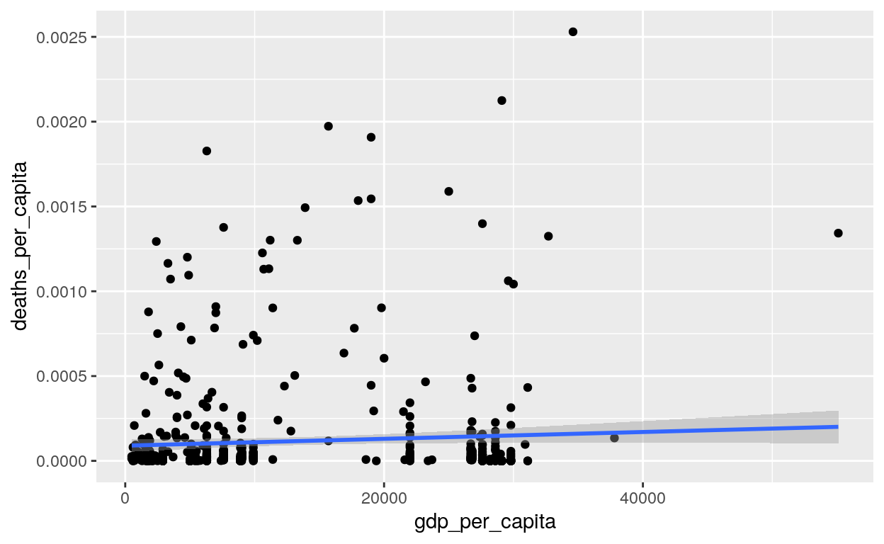

Mais transformações para formato `Tidy Data` com `{tidyr}`

O tidyr tem o famoso drop_na(). Então se vocês forem usar o drop_na() junto com o dplyr não esqueçam do library(tidyr).

OBS: vocês podem importar TODO o {tidyverse} de uma vez só com o library(tidyverse)

Em especial temos as funções pivot_longer() e pivot_wider():

Dataset tidyr::relig_income
Dataset tidyr::billboard
Dataset tidyr::fish_encounters

library(tidyr)
relig_income %>% 
  pivot_longer(!religion,
               names_to = "income",
               values_to = "count") %>% 
  mutate(across(where(is.character), as.factor)) %>% 
  filter(!str_detect(income, "Don't know")) %>% 
  count(religion, income, wt = count, sort = TRUE)

# A tibble: 162 × 3
   religion         income       n
   <fct>            <fct>    <dbl>
 1 Evangelical Prot $50-75k   1486
 2 Catholic         $50-75k   1116
 3 Mainline Prot    $50-75k   1107
 4 Evangelical Prot $20-30k   1064
 5 Evangelical Prot $30-40k    982
 6 Catholic         $75-100k   949
 7 Evangelical Prot $75-100k   949
 8 Mainline Prot    $75-100k   939
 9 Evangelical Prot $40-50k    881
10 Evangelical Prot $10-20k    869
# … with 152 more rows

billboard %>% 
  pivot_longer(
    cols = starts_with("wk"),
    names_to = "week",
    values_to = "rank",
    values_drop_na = TRUE
  ) %>% 
  group_by(artist) %>% 
  summarise(
    n = n(),
    median_rank = median(rank)) %>% 
  arrange(-n, median_rank)

# A tibble: 228 × 3
   artist                  n median_rank
   <chr>               <int>       <dbl>
 1 Creed                 104        28.5
 2 Lonestar               95        38  
 3 Destiny's Child        92        13  
 4 N'Sync                 74        12  
 5 Sisqo                  74        25.5
 6 3 Doors Down           73        42  
 7 Jay-Z                  73        45  
 8 Aguilera, Christina    67        17  
 9 Hill, Faith            67        28  
10 Houston, Whitney       67        54  
# … with 218 more rows

fish_encounters %>%
  pivot_wider(
    names_from = station,
    values_from = seen,
    values_fill = 0
  ) %>% 
  pivot_longer(!fish, names_to = "station", values_to = "seen")

# A tibble: 209 × 3
   fish  station  seen
   <fct> <chr>   <int>
 1 4842  Release     1
 2 4842  I80_1       1
 3 4842  Lisbon      1
 4 4842  Rstr        1
 5 4842  Base_TD     1
 6 4842  BCE         1
 7 4842  BCW         1
 8 4842  BCE2        1
 9 4842  BCW2        1
10 4842  MAE         1
# … with 199 more rows

Além do unnest_wider() e unnest_longer():

Dataset repurrrsive::got_chars

library(repurrrsive)
chars <- tibble(char = got_chars)
chars %>%
  unnest_wider(char) %>% 
  select(name, books, tvSeries) %>% 
  pivot_longer(!name, names_to = "media") %>% 
  unnest_longer(value) %>% 
  filter(media == "tvSeries") %>% 
  extract(value, "season", "(\\d{1})", convert = TRUE)

# A tibble: 102 × 3
   name             media    season
   <chr>            <chr>     <int>
 1 Theon Greyjoy    tvSeries      1
 2 Theon Greyjoy    tvSeries      2
 3 Theon Greyjoy    tvSeries      3
 4 Theon Greyjoy    tvSeries      4
 5 Theon Greyjoy    tvSeries      5
 6 Theon Greyjoy    tvSeries      6
 7 Tyrion Lannister tvSeries      1
 8 Tyrion Lannister tvSeries      2
 9 Tyrion Lannister tvSeries      3
10 Tyrion Lannister tvSeries      4
# … with 92 more rows

Uma outra maneira

chars %>%
  unnest_wider(char) %>% 
  select(name, books, tvSeries) %>% 
  pivot_longer(!name, names_to = "media") %>% 
  unnest_longer(value) %>% 
  filter(media == "tvSeries") %>% 
  separate(value, into = c(NA, "season"), sep = " ", fill = "right")

# A tibble: 102 × 3
   name             media    season
   <chr>            <chr>    <chr> 
 1 Theon Greyjoy    tvSeries 1     
 2 Theon Greyjoy    tvSeries 2     
 3 Theon Greyjoy    tvSeries 3     
 4 Theon Greyjoy    tvSeries 4     
 5 Theon Greyjoy    tvSeries 5     
 6 Theon Greyjoy    tvSeries 6     
 7 Tyrion Lannister tvSeries 1     
 8 Tyrion Lannister tvSeries 2     
 9 Tyrion Lannister tvSeries 3     
10 Tyrion Lannister tvSeries 4     
# … with 92 more rows

Extras

Converter verbos `{dplyr}` em SQL com o `{dbplyr}`

library(dplyr, warn.conflicts = FALSE)

con <- DBI::dbConnect(RSQLite::SQLite(), ":memory:")
copy_to(con, mtcars)

mtcars2 <- tbl(con, "mtcars")

Posso muito bem converter verbos {dplyr} para SQL (para todos os amantes de SQL)

summary <- mtcars2 %>% 
  group_by(cyl) %>% 
  summarise(mpg = mean(mpg, na.rm = TRUE)) %>% 
  arrange(-mpg)

summary %>% show_query()

<SQL>
SELECT `cyl`, AVG(`mpg`) AS `mpg`
FROM `mtcars`
GROUP BY `cyl`
ORDER BY -`mpg`

summary %>% collect()

# A tibble: 3 × 2
    cyl   mpg
  <dbl> <dbl>
1     4  26.7
2     6  19.7
3     8  15.1

Big Data com `{arrow}`

Ambiente

sessionInfo()

R version 4.2.2 (2022-10-31)
Platform: x86_64-pc-linux-gnu (64-bit)
Running under: Ubuntu 22.04.1 LTS

Matrix products: default
BLAS:   /usr/lib/x86_64-linux-gnu/openblas-pthread/libblas.so.3
LAPACK: /usr/lib/x86_64-linux-gnu/openblas-pthread/libopenblasp-r0.3.20.so

locale:
 [1] LC_CTYPE=en_US.UTF-8       LC_NUMERIC=C              
 [3] LC_TIME=en_US.UTF-8        LC_COLLATE=en_US.UTF-8    
 [5] LC_MONETARY=en_US.UTF-8    LC_MESSAGES=en_US.UTF-8   
 [7] LC_PAPER=en_US.UTF-8       LC_NAME=C                 
 [9] LC_ADDRESS=C               LC_TELEPHONE=C            
[11] LC_MEASUREMENT=en_US.UTF-8 LC_IDENTIFICATION=C       

attached base packages:
[1] stats     graphics  grDevices utils     datasets  methods  
[7] base     

other attached packages:
[1] repurrrsive_1.1.0 ggplot2_3.4.1     stringr_1.5.0    
[4] tidyr_1.3.0       janitor_2.2.0     dplyr_1.1.0      
[7] readr_2.1.4       magrittr_2.0.3    tibble_3.1.8     

loaded via a namespace (and not attached):
 [1] lubridate_1.9.2  lattice_0.20-45  png_0.1-8       
 [4] assertthat_0.2.1 rprojroot_2.0.3  digest_0.6.31   
 [7] utf8_1.2.3       R6_2.5.1         RSQLite_2.3.0   
[10] evaluate_0.20    highr_0.10       pillar_1.8.1    
[13] rlang_1.0.6      rstudioapi_0.14  blob_1.2.3      
[16] jquerylib_0.1.4  Matrix_1.5-1     rmarkdown_2.20  
[19] labeling_0.4.2   splines_4.2.2    bit_4.0.5       
[22] munsell_0.5.0    compiler_4.2.2   xfun_0.37       
[25] pkgconfig_2.0.3  mgcv_1.8-41      htmltools_0.5.4 
[28] downlit_0.4.2    tidyselect_1.2.0 bookdown_0.32   
[31] fansi_1.0.4      dbplyr_2.3.0     crayon_1.5.2    
[34] tzdb_0.3.0       withr_2.5.0      grid_4.2.2      
[37] nlme_3.1-160     jsonlite_1.8.4   gtable_0.3.1    
[40] lifecycle_1.0.3  DBI_1.1.3        scales_1.2.1    
[43] cli_3.6.0        stringi_1.7.12   vroom_1.6.1     
[46] cachem_1.0.6     farver_2.1.1     snakecase_0.11.0
[49] bslib_0.4.2      ellipsis_0.3.2   generics_0.1.3  
[52] vctrs_0.5.2      distill_1.5      tools_4.2.2     
[55] bit64_4.0.5      glue_1.6.2       purrr_1.0.1     
[58] hms_1.1.2        parallel_4.2.2   fastmap_1.1.0   
[61] yaml_2.3.7       timechange_0.2.0 colorspace_2.1-0
[64] memoise_2.0.1    knitr_1.42       sass_0.4.5

Manipulação de Dados

O que é Tidy Data?

O pipe `%>%`

Como ler dados com o `{readr}`

`col_types` – O argumento que eu mais uso em `read_*()`

Manipulação de dados com o `{dplyr}`

Selecionar Variáveis – `dplyr::select()`

Ordenar variáveis com `dplyr::arrange()`

Frequencias com `dplyr::count()`

Manipular Variáveis – `dplyr::mutate()`

`dplyr::if_else` e `dplyr::case_when`

Agrupar e Sumarizar Variáveis – `dplyr::group_by()` e `dplyr::summarise()`

Joins com `dplyr::join*`

Mais transformações para formato `Tidy Data` com `{tidyr}`

Extras

Converter verbos `{dplyr}` em SQL com o `{dbplyr}`

Big Data com `{arrow}`

Ambiente

Corrections

Reuse

Citation

Manipulação de Dados

O que é Tidy Data?

O pipe %>%

Como ler dados com o {readr}

col_types – O argumento que eu mais uso em read_*()

Manipulação de dados com o {dplyr}

Selecionar Variáveis – dplyr::select()

Ordenar variáveis com dplyr::arrange()

Frequencias com dplyr::count()

Manipular Variáveis – dplyr::mutate()

dplyr::if_else e dplyr::case_when

Agrupar e Sumarizar Variáveis – dplyr::group_by() e dplyr::summarise()

Joins com dplyr::join*

Mais transformações para formato Tidy Data com {tidyr}

Extras

Converter verbos {dplyr} em SQL com o {dbplyr}

Big Data com {arrow}

Ambiente

Corrections

Reuse

Citation

O pipe `%>%`

Como ler dados com o `{readr}`

`col_types` – O argumento que eu mais uso em `read_*()`

Manipulação de dados com o `{dplyr}`

Selecionar Variáveis – `dplyr::select()`

Ordenar variáveis com `dplyr::arrange()`

Frequencias com `dplyr::count()`

Manipular Variáveis – `dplyr::mutate()`

`dplyr::if_else` e `dplyr::case_when`

Agrupar e Sumarizar Variáveis – `dplyr::group_by()` e `dplyr::summarise()`

Joins com `dplyr::join*`

Mais transformações para formato `Tidy Data` com `{tidyr}`

Converter verbos `{dplyr}` em SQL com o `{dbplyr}`

Big Data com `{arrow}`