What is Bayesian Statistics?

Bayesian statistics is an approach to inferential statistics based on Bayes' theorem, where available knowledge about parameters in a statistical model is updated with the information in observed data. The background knowledge is expressed as a prior distribution and combined with observational data in the form of a likelihood function to determine the posterior distribution. The posterior can also be used for making predictions about future events.

Bayesian statistics is a departure from classical inferential statistics that prohibits probability statements about parameters and is based on asymptotically sampling infinite samples from a theoretical population and finding parameter values that maximize the likelihood function. Mostly notorious is null-hypothesis significance testing (NHST) based on p-values. Bayesian statistics incorporate uncertainty (and prior knowledge) by allowing probability statements about parameters, and the process of parameter value inference is a direct result of the Bayes' theorem.

Bayesian statistics is revolutionizing all fields of evidence-based science^[1] (van de Schoot et al., 2021). Dissatisfaction with traditional methods of statistical inference (frequentist statistics) and the advent of computers with exponential growth in computing power^[2] provided a rise in Bayesian statistics because it is an approach aligned with the human intuition of uncertainty, robust to scientific malpractices, but computationally intensive.

But before we get into Bayesian statistics, we have to talk about probability: the engine of Bayesian inference.

What is Probability?

PROBABILITY DOES NOT EXIST!

de Finetti (1974)^[3]

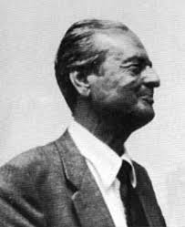
These are the first words in the preface to the famous book by Bruno de Finetti (figure below), one of the most important probability mathematician and philosopher. Yes, probability does not exist. Or rather, probability as a physical quantity, objective chance, does NOT exist. De Finetti showed that, in a precise sense, if we dispense with the question of objective chance nothing is lost. The mathematics of inductive reasoning remains exactly the same.

Consider tossing a weighted coin. The attempts are considered independent and, as a result, exhibit another important property: the order does not matter. To say that order does not matter is to say that if you take any finite sequence of heads and tails and exchange the results however you want, the resulting sequence will have the same probability. We say that this probability is invariant under permutations.

Or, to put it another way, the only thing that matters is the relative frequency. Result that have the same frequency of heads and tails consequently have the same probability. The frequency is considered a sufficient statistic. Saying that order doesn't matter or saying that the only thing that matters is frequency are two ways of saying exactly the same thing. This property is called exchangeability by de Finetti. And it is the most important property of probability that makes it possible for us to manipulate it mathematically (or philosophically) even if it does not exist as a physical "thing".

Still developing the argument:

"Probabilistic reasoning - always understood as subjective - stems merely from our being uncertain about something. It makes no difference whether the uncertainty relates to an unforeseeable future ^[4], or to an unnoticed past, or to a past doubtfully reported or forgotten ^[5]... The only relevant thing is uncertainty - the extent of our own knowledge and ignorance. The actual fact of whether or not the events considered are in some sense determined, or known by other people, and so on, is of no consequence." (de Finetti, 1974)

In conclusion: no matter what the probability is, you can use it anyway, even if it is an absolute frequency (ex: probability that I will ride my bike naked is ZERO because the probability that an event that never occurred will occur in the future it is ZERO) or a subjective guess (ex: maybe the probability is not ZERO, but 0.00000000000001; very unlikely, but not impossible).

Mathematical Definition

With the philosophical intuition of probability elaborated, we move on to mathematical intuitions. The probability of an event is a real number^[6], $\in \mathbb{R}$ between 0 and 1, where, roughly, 0 indicates the impossibility of the event and 1 indicates the certainty of the event. The greater the likelihood of an event, the more likely it is that the event will occur. A simple example is the tossing of a fair (impartial) coin. Since the coin is fair, both results ("heads" and "tails") are equally likely; the probability of "heads" is equal to the probability of "tails"; and since no other result is possible^[7], the probability of "heads" or "tails" is $\frac{1}{2}$ (which can also be written as 0.5 or 50%).

Regarding notation, we define $A$ as an event and $P(A)$ as the probability of event $A$, thus:

$$\{P(A) \in \mathbb{R} : 0 \leq P(A) \leq 1 \}.$$

This means the "probability of the event to occur is the set of all real numbers between 0 and 1; including 0 and 1". In addition, we have three axioms^[8], originated from Kolmogorov(1933) (figure below):

1. Non-negativity: For all $A$, $P(A) \geq 0$. Every probability is positive (greater than or equal to zero), regardless of the event.

2. Additivity: For two mutually exclusive $A$ and $B$ (cannot occur at the same time^[9]): $P(A) = 1 - P(B)$ and $P(B) = 1 - P(A)$.

3. Normalization: The probability of all possible events $A_1, A_2, \dots$ must add up to 1: $\sum_{n \in \mathbb{N}} P(A_n) = 1$.

With these three simple (and intuitive) axioms, we are able to derive and construct all the mathematics of probability.

Conditional Probability

An important concept is the conditional probability that we can define as the "probability that one event will occur if another has occurred or not". The notation we use is $P(A \mid B)$, which reads as "the probability that we have observed $A$ given we have already observed $B$".

A good example is the Texas Hold'em Poker game, where the player receives two cards and can use five "community cards" to set up his "hand". The probability that you are dealt a King ($K$) is $\frac{4}{52}$:

$$P(K) = \left(\frac{4}{52}\right) = \left(\frac{1}{13}\right) .$$

And the probability of being dealt an Ace is also the same as (2), $\frac{4}{52}$:

$$P(A) = \left(\frac{4}{52}\right) = \left(\frac{1}{13}\right) .$$

However, the probability that you are dealt a King as a second card since you have been dealt an Ace as a first card is:

$$P(K \mid A) = \left(\frac{4}{51}\right) .$$

Since we have one less card ($52 - 1 = 51$) because you have been dealt already an Ace (thus $A$ has been observed), we have 4 Kings still in the deck, so the (4) is $\frac{4}{51}$.

Joint Probability

Conditional probability leads us to another important concept: joint probability. Joint probability is the "probability that two events will both occur". Continuing with our Poker example, the probability that you will receive two cards, Ace ($A$) and a King ($K$) as two starting cards is:

$$\begin{aligned} P(A,K) &= P(A) \cdot P(K \mid A) \\ &= P \left(\frac{1}{13}\right) \cdot P \left(\frac{4}{51}\right)\\ &= P \left(\frac{4}{51 \cdot 13}\right) \\ &\approx 0.006 . \end{aligned}$$

Note that $P(A,K) = P(K,A)$:

$$\begin{aligned} P(K,A) &= P(K) \cdot P(A \mid K) \\ &= P \left(\frac{1}{13}\right) \cdot P \left(\frac{4}{51}\right)\\ &= P \left(\frac{4}{51 \cdot 13}\right) \\ &\approx 0.006 . \end{aligned}$$

But this symmetry does not always exist (in fact it very rarely exists). The identity we have is as follows:

$$P(A) \cdot P(K \mid A) = P(K) \cdot P(A \mid K) .$$

So this symmetry only exists when the baseline rates for conditional events are equal:

$$P(A) = P(K).$$

Which is what happens in our example.

Conditional Probability is not "commutative"

$$P(A \mid B) \neq P(B \mid A)$$

Let's see a practical example. For example, I’m feeling good and start coughing in line at the supermarket. What do you think will happen? Everyone will think I have COVID, which is equivalent to thinking about $P(\text{cough} \mid \text{covid})$. Seeing the most common symptoms of COVID, if you have COVID, the chance of coughing is very high. But we actually cough a lot more often than we have COVID – $P(\text{cough}) \neq P(\text{COVID})$, so:

$$P(\text{COVID} \mid \text{cough}) \neq P(\text{cough} \mid \text{COVID}) .$$

Bayes' Theorem

This is the last concept of probability that we need to address before diving into Bayesian statistics, but it is the most important. Note that it is not a semantic coincidence that Bayesian statistics and Bayes' theorem have the same prefix.

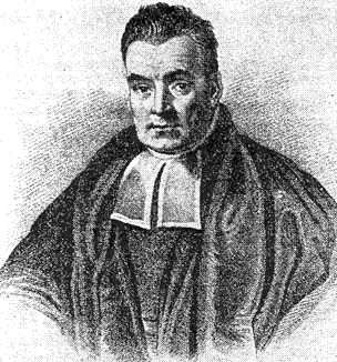
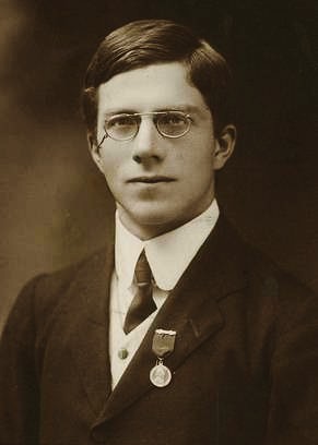
Thomas Bayes (1701 - 1761, figure below) was an English Presbyterian statistician, philosopher and minister known for formulating a specific case of the theorem that bears his name: Bayes' theorem. Bayes never published what would become his most famous accomplishment; his notes were edited and published after his death by his friend Richard Price^[10]. In his later years, Bayes was deeply interested in probability. Some speculate that he was motivated to refute David Hume's argument against belief in miracles based on evidence from the testimony in "An Inquiry Concerning Human Understanding".

Let's move on to Theorem. Remember that we have the following identity in probability:

$$\begin{aligned} P(A,B) &= P(B,A) \\ P(A) \cdot P(B \mid A) &= P(B) \cdot P(A \mid B) . \end{aligned}$$

Ok, now move $P(B)$ in the right of (11) to the left as a division:

$$\begin{aligned} P(A) \cdot P(B \mid A) &= \overbrace{P(B)}^{\text{this goes to $\leftarrow$}} \cdot P(A \mid B) \\ &\\ \frac{P(A) \cdot P(B \mid A)}{P(B)} &= P(A \mid B) \\ P(A \mid B) &= \frac{P(A) \cdot P(B \mid A)}{P(B)}. \end{aligned}$$

And the final result is:

$$P(A \mid B) = \frac{P(A) \cdot P(B \mid A)}{P(B)}.$$

Bayesian statistics uses this theorem as inference engine of parameters of a model conditioned on observed data.

Discrete vs Continuous Parameters

Everything that has been exposed so far is based on the assumption that the parameters are discrete. This was done in order to provide a better intuition of what is probability. We do not always work with discrete parameters. The parameters can be continuous, for example: age, height, weight, etc. But don't despair, all the rules and axioms of probability are also valid for continuous parameters. The only thing we have to do is to exchange all the sums $\sum$ for integrals $\int$. For example, the third axiom of Normalization for continuous random variables becomes:

$$\int_{x \in X} p(x) dx = 1 .$$

Bayesian Statistics

Now that you know what probability is and what Bayes' theorem is, I will propose the following model:

$$\underbrace{P(\theta \mid y)}_{\text{Posterior}} = \frac{\overbrace{P(y \mid \theta)}^{\text{Likelihood}} \cdot \overbrace{P(\theta)}^{\text{Prior}}}{\underbrace{P(y)}_{\text{Normalizing Constant}}} ,$$

where:

• $\theta$ – parameter(s) of interest;

• $y$ – observed data;

• Prior – previous probability of the parameter value(s)^[11] $\theta$;

• Likelihood – probability of the observed data $y$ conditioned on the parameter value(s) $\theta$;

• Posterior – posterior probability of the parameter value(s) $\theta$ after observing the data $y$; and

• Normalizing Constant – $P(y)$ does not make intuitive sense. This probability is transformed and can be interpreted as something that exists only so that the result of $P(y \mid \theta) P(\theta)$ is somewhere between 0 and 1 – a valid probability by the axioms. We will talk more about this constant in 5. Markov Chain Monte Carlo (MCMC).

Bayesian statistics allow us to directly quantify the uncertainty related to the value of one or more parameters of our model conditioned to the observed data. This is the main feature of Bayesian statistics, for we are directly estimating $P (\theta \mid y)$ using Bayes' theorem. The resulting estimate is totally intuitive: it simply quantifies the uncertainty we have about the value of one or more parameters conditioned on the data, the assumptions of our model (likelihood) and the previous probability(prior) we have about such values.

Frequentist Statistics

To contrast with Bayesian statistics, let's look at the frequentist statistics, also known as "classical statistics". And already take notice: it is not something intuitive like the Bayesian statistics.

For frequentist statistics, the researcher is prohibited from making probabilistic conjectures about parameters. Because they are not uncertain, quite the contrary they are determined quantities. The only issue is that we do not directly observe the parameters, but they are deterministic and do not allow any margin of uncertainty. Therefore, for the frequentist approach, parameters are unobserved amounts of interest in which we do not make probabilistic conjectures.

What, then, is uncertain in frequentist statistics? Short answer: the observed data. For the frequentist approach, the sample is uncertain. Thus, we can only make probabilistic conjectures about our sample. Therefore, the uncertainty is expressed in the probability that I will obtain data similar to those that I obtained if I sampled from a population of interest infinite samples of the same size as my sample^[12]. Uncertainty is conditioned by a frequentist approach, in other words, uncertainty only exists only if I consider an infinite sampling process and extract a frequency from that process. The probability only exists if it represents a frequency. Frequentist statistics is based on an "infinite sampling process of a population that I have never seen", strange that it may sounds.

For the frequentist approach, there is no posterior or prior probability since both involve parameters, and we saw that this is a no-no on frequentist soil. Everything that is necessary for statistical inference is contained within likelihood^[13].

In addition, for reasons of ease of computation, since most of these methods were invented in the first half of the 20th century (without any help of a computer), only the parameter value(s) that maximize(s) the likelihood function is(are) computed^[14]. From this optimization process we extracted the mode of the likelihood function (i.e. maximum value). The maximum likelihood estimate (MLE) is(are) the parameter value(s) so that a $N$-sized sample randomly sampled from a population (i.e. the data you've collected) is the most likely $N$-sized sample from that population. All other potential samples that could be extracted from this population will have a worse estimate than the sample you actually have^[15]. In other words, we are conditioning the parameter value(s) on the observed data from the assumption that we are sampling infinite $N$-sized samples from a theoretical population and treating the parameter values as fixed and our sample as random (or uncertain).

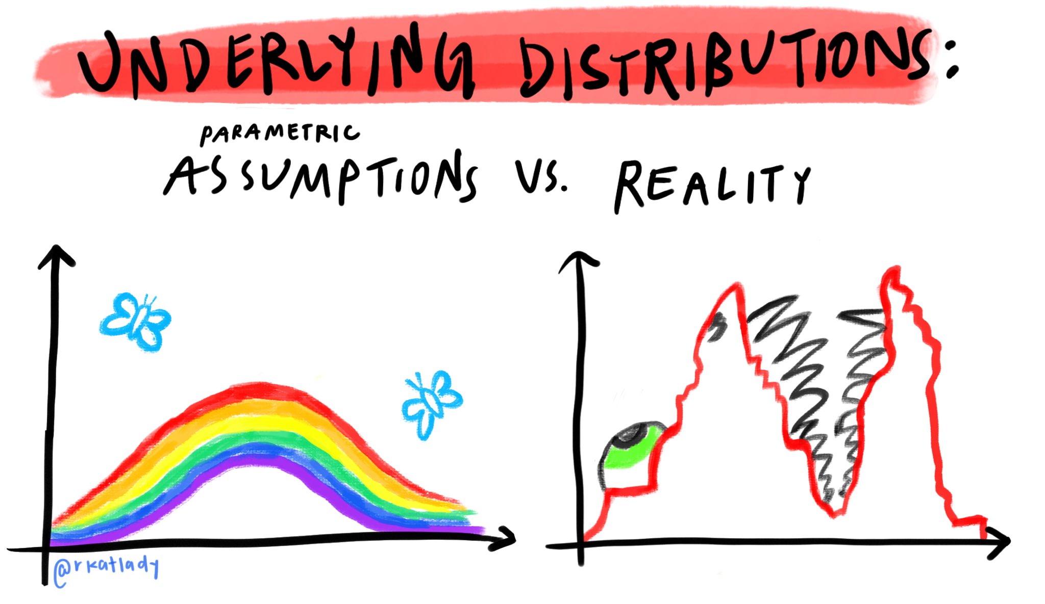
The mode works perfectly in the fairytale world, which assumes that everything follows a normal distribution, in which the mode is equal to the median and to the mean – $\text{mean} = \text{median} = \text{mode}$. There is only one problem, this assumption is rarely true (see figure below), especially when we are dealing with multiple parameters with complex relationships between them (complex models).

A brief sociological and computational explanation is worthwhile of why frequentist (classical) statistics prohibit probabilistic conjectures about parameters and we are only left with optimizing (finding the maximum value of a function) rather than approximating or estimating a complete likelihood density (in other words, "to pull up the whole file" of the likelihood verisimilitude instead of just the mode).

On the sociological side of things, science at the beginning of the 20th century assumed that it should be strictly objective and all subjectivity must be banned. Therefore, since the estimation of the a posterior probability of parameters involves elucidating an a prior probability of parameters, such a method should not be allowed in science, as it brings subjectivity (we know today that nothing in human behavior is purely objective, and subjectivity permeates all human endeavors).

Regarding the computational side of things, in the 1930s without computers it was much easier to use strong assumptions about the data to get a value from a statistical estimation using mathematical derivations than to calculate the statistical estimation by hand without depending on such assumptions. For example: Student's famous $t$ test is a test that indicates when we can reject that the mean of a certain parameter of interest between two groups is equal (famous null hypothesis - $H_0$). This test starts from the assumption that if the parameter of interest is distributed according to a normal distribution (assumption 1 – normality of the dependent variable), if the variance of the parameter of interest varies homogeneously between groups (assumption 2 – homogeneity of the variances), and if the number of observations in the two groups are similar (assumption 3 – homogeneity of the size of the groups) the difference between the groups weighted by the variance of the groups follows a Student-$t$ distribution (hence the name of the test).

So statistical estimation comes down to calculating the average of two groups, the variance of both groups for a parameter of interest and looking for the associated $p$-value in a table and see if we can reject the $H_0$. This was valid when everything we had to do was calculated by hand. Today, with a computer 1 million times more powerful than the Apollo 11 computer (one that took humanity to the moon) in your pocket ^[2], I don't know if it is still valid.

$p$-values

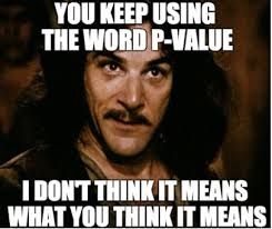
$p$-values are hard to understand, $p < 0.05$.

Since I've mentioned the $p$ word, let me explain what it is. First, the correct^[16] statistics textbook definition:

$p$-value is the probability of obtaining test results at least as extreme as the results actually observed, under the assumption that the null hypothesis is correct.

Unfortunately with frequentist statistics you have to choose one of two qualities for explanations: intuitive or accurate^[17].

If you write this definition in any test, book or scientific paper, you are 100% accurate and correct in defining what a $p$-value is. Now, understanding this definition is complicated. For that, let's break this definition down into parts for a better understanding:

• "probability of obtaining test results..": notice that $p$-values are related your data and not your theory or hypothesis.

• "...at least as extreme as the results actually observed...": "at least as extreme" implies defining a threshold for the characterization of some relevant finding, which is commonly called $\alpha$. We generally stipulate alpha at 5% ($\alpha = 0.05$) and anything more extreme than alpha (ie less than 5%) we characterize as significant.

• "... under the assumption that the null hypothesis is correct.": every statistical test that has a $p$-value has a null hypothesis (usually written as $H_0$). Null hypotheses, always have to do with some null effect. For example, the null hypothesis of the Shapiro-Wilk and Komolgorov-Smirnov test is "the data is distributed according to a Normal distribution" and that of the Levene test is "the group variances are equal". Whenever you see a $p$-value, ask yourself: "What is the null hypothesis that this test assumes is correct?".

To understand the $p$-value any statistical test first find out what is the null hypothesis behind that test. The definition of $p$-value will not change. In every test it is always the same. What changes with the test is the null hypothesis. Each test has its $H_0$. For example, some common statistical tests ($\text{D}^*$ = data at least as extreme as the results actually observed):

• $t$ Test: $P(\text{D}^* \mid \text{the difference between groups are zero})$

• ANOVA: $P(\text{D}^* \mid \text{there is no difference between groups})$

• Regression: $P(\text{D}^* \mid \text{the coefficient is zero})$

• Shapiro-Wilk: $P(\text{D}^* \mid \text{the sample follows a normal distribution})$

$p$-value is the probability of the data you obtained given that the null hypothesis is true. For those who like mathematical formalism: $p = P(\text{D}^* \mid H_0)$. In English, this expression means "the probability of $\text{D}^*$ conditioned to $H_0$". Before moving on to some examples and attempts to formalize an intuition about $p$-values, it is important to note that $p$-values say something about data and not hypotheses. For $p$-value, the null hypothesis is true, and we are only evaluating whether the data conforms to this null hypothesis or not. If you leave this tutorial armed with this intuition, the world will be rewarded with researchers better prepared to qualify and interpret evidence ($p <0.05$).

$p$-values – A historical perspective

There is no way to understand $p$-values ​​if we do not understand its origins and historical trajectory. The first mention of the term was made by statistician Ronald Fisher^[18] (figure below). In 1925, Fisher (Fisher, 1925) defined the $p$-value as an "index that measures the strength of the evidence against the null hypothesis". To quantify the strength of the evidence against the null hypothesis, Fisher defended "$p <0.05$ (5% significance) as a standard level to conclude that there is evidence against the tested hypothesis, although not as an absolute rule". Fisher did not stop there but rated the strength of the evidence against the null hypothesis. He proposed "if $p$ is between 0.1 and 0.9 there is certainly no reason to suspect the hypothesis tested. If it is below 0.02 it is strongly indicated that the hypothesis fails to account for the whole of the facts. We shall not often be astray if we draw a conventional line at 0.05". Since Fisher made this statement almost 100 years ago, the 0.05 threshold has been used by researchers and scientists worldwide and it has become ritualistic to use 0.05 as a threshold as if other thresholds could not be used or even considered.

After that, the threshold of 0.05, now established as unquestionable, strongly influenced statistics and science. But there is no reason against adopting other thresholds ($\alpha$) like 0.1 or 0.01 (Lakens et al., 2018). If well argued, the choice of thresholds other than 0.05 can be welcomed by editors, reviewers and advisors. Since the $p$-value is a probability, it is a continuous quantity. There is no reason to differentiate a $p$ of 0.049 against a $p$ of 0.051. Robert Rosenthal, a psychologist already said "God loves $p$ 0.06 as much as a $p$ 0.05" (Rosnow & Rosenthal, 1989).

In the last year of his life, Fisher published an article (Fisher, 1962) examining the possibilities of Bayesian methods, but with a prior probabilities to be determined experimentally. Some authors even speculate (Jaynes, 2003) that if Fisher were alive today, he would probably be a "Bayesian".

What the $p$-value is not

With the definition and a well-anchored intuition of what $p$-value is, we can move on to what the $p$-value is not!

1. $p$-value is not the probability of the null hypothesis - Famous confusion between $P(D \mid H_0)$ and $P(H_0 \mid D)$. $p$-value is not the probability of the null hypothesis, but the probability of the data you obtained. To get the $P(H_0 \mid D)$ you need Bayesian statistics.

2. $p$-value is not the probability of the data being produced by chance - No! Nobody said anything of "being produced by chance". Again: $p$-value is the probability to get results at least as extreme as those that were observed, given that the null hypothesis is true.

3. $p$-value measures the size of the effect of a statistical test - Also wrong... $p$-value does not say anything about the size of the effect. Just about whether the observed data differs from what is expected under the null hypothesis. It is clear that large effects are more likely to be statistically significant than small effects. But this is not a rule and never judge a finding by its $p$-value, but by its effect size. In addition, $p$-values ​​can be "hacked" in a number of ways (Head et al., 2015) and often their value is a direct consequence of the sample size.

Confidence Intervals

To conclude, let's talk about the famous confidence intervals, which are not a measure that quantifies the uncertainty of the value of a parameter (remember probabilistic conjectures about parameters are prohibited in frequentist-land). Wait for it! Here is the definition of confidence intervals:

"An X% confidence interval for a parameter $\theta$ is an interval $(L, U)$ generated by a procedure that in repeated sampling has an X% probability of containing the true value of $\theta$, for all possible values of $\theta$."

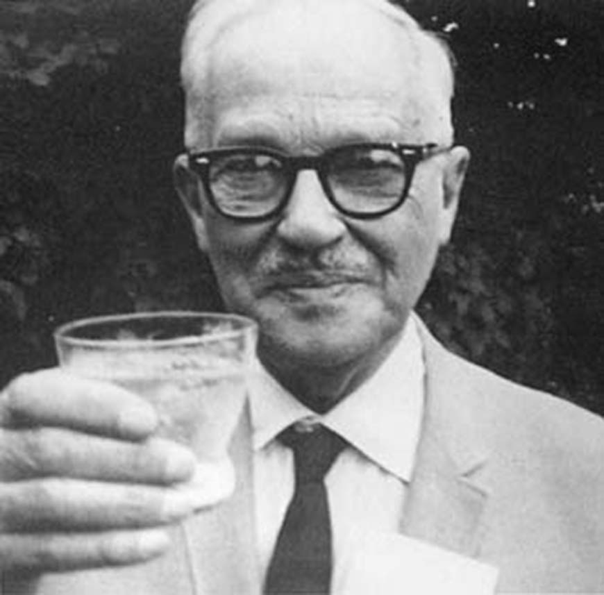
Jerzy Neyman, the "father" of confidence intervals (see figure below) (Neyman, 1937).

Again the idea of sampling an infinite number of times from a population you have never seen. For example: let's say that you performed a statistical analysis to compare the effectiveness of a public policy in two groups and you obtained the difference between the average of those groups. You can express this difference as a confidence interval. We generally choose 95% confidence (since it is analogous as $p < 0.05$). You then write in your paper that the "observed difference between groups is 10.5 - 23.5 (95% CI)." This means that approximately 95 studies out of 100 would compute a confidence interval that contains the true mean difference –- but it says nothing about which ones those are (whereas the data might). In other words, 95% is not the probability of obtaining data such that the estimate of the true parameter is contained in the interval that we obtained, it is the probability of obtaining data such that, if we compute another confidence interval in the same way, it contains the true parameter. The interval that we got in this particular instance is irrelevant and might as well be thrown away.

Confidence Intervals (Frequentist) vs Credible Intervals (Bayesian)

Bayesian statistics have a concept similar to the confidence intervals of frequentist statistics. This concept is called credibility interval. And, unlike the confidence interval, its definition is intuitive. Credibility interval measures an interval in which we are sure that the value of the parameter of interest is, based on the likelihood conditioned on the observed data - $P(y \mid \theta)$; and the prior probability of the parameter of interest - $P(\theta)$. It is basically a "slice" of the posterior probability of the parameter restricted to a certain level of certainty. For example: a 95% credibility interval shows the interval that we are 95% sure that captures the value of our parameter of interest. That simple...

For example, see figure below, which shows a Log-Normal distribution with mean 0 and standard deviation 2. The green dot shows the maximum likelihood estimation (MLE) of the value of $\theta$ which is simply the mode of distribution. And in the shaded area we have the 50% credibility interval of the value of $\theta$, which is the interval between the 25% percentile and the 75% percentile of the probability density of $\theta$. In this example, MLE leads to estimated values that are not consistent with the actual probability density of the value of $\theta$.

using CairoMakie
using Distributions

d = LogNormal(0, 2)
range_d = 0:0.001:4
q25 = quantile(d, 0.25)
q75 = quantile(d, 0.75)
credint = range(q25; stop=q75, length=100)
f, ax, l = lines(
    range_d,
    pdf.(d, range_d);
    linewidth=3,
    axis=(; limits=(-0.2, 4.2, nothing, nothing), xlabel=L"\theta", ylabel="Density"),
)
scatter!(ax, mode(d), pdf(d, mode(d)); color=:green, markersize=12)
band!(ax, credint, 0.0, pdf.(d, credint); color=(:steelblue, 0.5))

Now an example of a multimodal distribution^[19]. The figure below shows a bimodal distribution with two modes 2 and 10^[20] The green dot shows the maximum likelihood estimation (MLE) of the value of $\theta$ which is the mode of distribution. See that even with 2 modes, maximum likelihood defaults to the highest mode^[21]. And in the shaded area we have the 50% credibility interval of the value of $\theta$, which is the interval between the 25% percentile and the 75% percentile of the probability density of $\theta$. In this example, estimation by maximum likelihood again lead us to estimated values ​​that are not consistent with the actual probability density of the value of $\theta$.

d1 = Normal(10, 1)
d2 = Normal(2, 1)
mix_d = [0.4, 0.6]
d = MixtureModel([d1, d2], mix_d)
range_d = -2:0.01:14
sim_d = rand(d, 10_000)
q25 = quantile(sim_d, 0.25)
q75 = quantile(sim_d, 0.75)
credint = range(q25; stop=q75, length=100)

f, ax, l = lines(
    range_d,
    pdf.(d, range_d);
    linewidth=3,
    axis=(;
        limits=(-2, 14, nothing, nothing),
        xticks=[0, 5, 10],
        xlabel=L"\theta",
        ylabel="Density",
    ),
)
scatter!(ax, mode(d2), pdf(d, mode(d2)); color=:green, markersize=12)
band!(ax, credint, 0.0, pdf.(d, credint); color=(:steelblue, 0.5))

Bayesian Statistics vs Frequentist Statistics

What we've seen so fat can be resumed in the table below:

	Bayesian Statistics	Frequentist Statistics
Data	Fixed – Non-random	Uncertain – Random
Parameters	Uncertain – Random	Fixed – Non-random
Inference	Uncertainty over parameter values	Uncertainty over a sampling procedure from an infinite population
Probability	Subjective	Objective (but with strong model assumptions)
Uncertainty	Credible Interval – $P(\theta \mid y)$	Confidence Interval – $P(y \mid \theta)$

Advantages of Bayesian Statistics

Finally, I summarize the main advantages of Bayesian statistics:

• Natural approach to express uncertainty

• Ability to incorporate prior information

• Greater model flexibility

• Complete posterior distribution of parameters

  • Confidence Intervals vs Credibility Intervals

• Natural propagation of uncertainty

And I believe that I also need to show the main disadvantage:

• Slow model estimation speed (30 seconds instead of 3 seconds using the frequentist approach)

The beginning of the end of Frequentist Statistics

Dear reader, know that you are at a time in history when Statistics is undergoing major changes. I believe that frequentist statistics, especially the way we qualify evidence and hypotheses with $p$-values, will transform in a "significant" way. Five years ago, the American Statistical Association (ASA, the world's largest professional statistical organization) published a statement on $p$-values (Wasserstein & Lazar, 2016). The statement says exactly what we talk about here. The main concepts of the null hypothesis significance test, and in particular $p$-values, fail to provide what researchers require of them. Despite what many statistical books, teaching materials and published articles say, $p$-values ​​below 0.05 do not "prove" the reality of anything. Nor, at this point, do the $p$-values ​​above 0.05 refute anything. ASA's statement has more than 3,600 citations causing significant impact. As an example, an international symposium was held in 2017 that led to a special open access edition of The American Statistician dedicated to practical ways to abandon $p <0.05$ (Wasserstein, Schirm & Lazar 2019).

Soon after, more attempts and claims followed. In September 2017, Nature Human Behavior published an editorial proposing that the significance level of the $p$-value be reduced from $0.05$ to $0.005$ (Benjamin et al., 2018). Several authors, including many highly influential and important statisticians, have argued that this simple step would help tackle the problem of the science replicability crisis, which many believe is the main consequence of the abusive use of $p$-values (Ioannidis, 2019). In addition, many have gone a step further and suggest that science discard once and for all $p$-values (Nature, 2019). Many suggest (myself included) that the main inference tool be Bayesian statistics (Amrhein, Greenland & McShane, 2019; Goodman, 2016; van de Schoot et al., 2021)

Turing

Turing (Ge, Xu & Ghahramani, 2018) is a probabilistic programming interface written in Julia (Bezanson, Edelman, Karpinski & Shah, 2017). It enables intuitive modeling syntax with flexible composable probabilistic programming inference. Turing supports a wide range of sampling based inference algorithms by combining model inference with differentiable programming interfaces in Julia. Yes, Julia is that amazing. The same differentiable stuff that you develop for optimization in neural networks you can plug it in to a probabilistic programming framework and it will work without much effort and boiler-plate code. Most importantly, Turing inference is composable: it combines Markov chain sampling operations on subsets of model variables, e.g. using a combination of a Hamiltonian Monte Carlo (HMC) engine and a particle Gibbs (PG) engine. This composable inference engine allows the user to easily switch between black-box style inference methods such as HMC, and customized inference methods.

I believe Turing is the most important and popular probabilistic language framework in Julia. It is what PyMC3 and Stan are for Python and R, but for Julia. Furthermore, you don't have to do "cartwheels" with Theano backends and tensors like in PyMC3 or learn a new language to declare your models like in Stan (or even have to debug C++ stuff). Turing is all Julia. It uses Julia arrays, Julia distributions, Julia autodiff, Julia plots, Julia random number generator, Julia MCMC algorithms etc. I think that developing and estimating Bayesian probabilistic models using Julia and Turing is powerful, intuitive, fun, expressive and allows easily new breakthroughs simply by being 100% Julia and embedded in Julia ecosystem. As discussed in 1. Why Julia?, having multiple dispatch with LLVM's JIT compilation allows us to combine code, types and algorithms in a very powerful and yet simple way. By using Turing in this context, a researcher (or a curious Joe) can develop new methods and extend the frontiers of Bayesian inference with new models, samplers, algorithms, or any mix-match of those.

Footnotes

[1]

personally, like a good Popperian, I don't believe there is science without being evidence-based; what does not use evidence can be considered as logic, philosophy or social practices (no less or more important than science, just a demarcation of what is science and what is not; eg, mathematics and law).

[2]	your smartphone (iPhone 12 - 4GB RAM) has 1,000,000x (1 million) more computing power than the computer that was aboard the Apollo 11 (4kB RAM) which took the man to the moon. Detail: this on-board computer was responsible for lunar module navigation, route and controls.

[3]	if the reader wants an in-depth discussion see Nau (2001).

[4]	my observation: related to the subjective Bayesian approach.

[5]	my observation: related to the objective frequentist approach.

[6]	a number that can be expressed as a point on a continuous line that originates from minus infinity and ends and plus infinity $(-\infty, +\infty)$; for those who like computing it is a floating point float ordouble.

[7]	i.e. the events are "mutually exclusive". That means that only $A$ or $B$ can occur in the whole sample space.

[8]

in mathematics, axioms are assumptions assumed to be true that serve as premises or starting points for the elaboration of arguments and theorems. Often the axioms are questionable, for example non-Euclidean geometry refutes Euclid's fifth axiom on parallel lines. So far there is no questioning that has supported the scrutiny of time and science about the three axioms of probability.

[9]	for example, the result of a given coin is one of two mutually exclusive events: heads or tails.

[10]

the formal name of the theorem is Bayes-Price-Laplace, as Thomas Bayes was the first to discover, Richard Price took his drafts, formalized in mathematical notation and presented to the Royal Society of London, and Pierre Laplace rediscovered the theorem without having had previous contact in the late 18th century in France by using probability for statistical inference with Census data in the Napoleonic era.

[11]	I will cover prior probabilities in the content of tutorial 4. How to use Turing.

[12]	I warned you that it was not intuitive...

[13]	something worth noting: likelihood also carries a lot of subjectivity.

[14]

for those who have a thing for mathematics (like myself), we calculate at which point of $\theta$ the derivative of the likelihood function is zero - $\mathcal{L}^\prime = 0$. So we are talking really about an optimization problem that for some likelihood functions we can have a closed-form analytical solution.

[15]	have I forgot to warn you that it is not so intuitive?

[16]	there are several statistics textbooks that have wrong definitions of what a $p$-value is. If you don't believe me, see Wasserstein & Lazar (2016).

[17]	this duality is attributed to Andrew Gelman – Bayesian statistician.

[18]

Ronald Fisher's personality and life controversy deserves a footnote. His contributions were undoubtedly crucial to the advancement of science and statistics. His intellect was brilliant and his talent already flourished young: before turning 33 years old he had proposed the maximum likelihood estimation method (MLE) (Stigler, 2007) and also created the concept of degrees of freedom when proposing a correction in Pearson's chi-square test (Baird, 1983). He also invented the Analysis of Variance (ANOVA) and was the first to propose randomization as a way of carrying out experiments, being considered the "father" of randomized clinical trials (RCTs). Not everything is golden in Fisher's life, he was a eugenicist and had a very strong view on ethnicity and race, advocating the superiority of certain ethnicities. Furthermore, he was extremely invariant, chasing, harming and mocking any critic of his theories and publications. What we see today in the monopoly of the Neyman-Pearson paradigm (Neyman & Pearson, 1933) with $p$-values ​​and null hypotheses the result of this Fisherian effort to silence critics and let only his voice echo.

[19]	which is not uncommon to see in the real world.

[20]	for the curious it is a mixture of two normal distributions both with standard deviation 1, but with different means. To complete it assigns the weights of 60% for the distribution with an average of 2 and 40% for the distribution with an average of 10.

[21]	to be more precise, estimation by maximum likelihood in non-convex functions cannot find an analytical solution and, if we are going to use another iterative maximization procedure, there is a risk of it becoming stuck in the second – lower-valued – mode of distribution.

References

Amrhein, V., Greenland, S., & McShane, B. (2019). Scientists rise up against statistical significance. Nature, 567(7748), 305–307. https://doi.org/10.1038/d41586-019-00857-9

Baird, D. (1983). The fisher/pearson chi-squared controversy: A turning point for inductive inference. The British Journal for the Philosophy of Science, 34(2), 105–118.

Benjamin, D. J., Berger, J. O., Johannesson, M., Nosek, B. A., Wagenmakers, E.-J., Berk, R., … Johnson, V. E. (2018). Redefine statistical significance. Nature Human Behaviour, 2(1), 6–10. https://doi.org/10.1038/s41562-017-0189-z

Bezanson, J., Edelman, A., Karpinski, S., & Shah, V. B. (2017). Julia: A fresh approach to numerical computing. SIAM Review, 59(1), 65–98.

de Finetti, B. (1974). Theory of Probability. New York: John Wiley & Sons.

Eckhardt, R. (1987). Stan Ulam, John von Neumann, and the Monte Carlo Method. Los Alamos Science, 15(30), 131–136.

Fisher, R. A. (1925). Statistical methods for research workers. Oliver; Boyd.

Fisher, R. A. (1962). Some Examples of Bayes’ Method of the Experimental Determination of Probabilities A Priori. Journal of the Royal Statistical Society. Series B (Methodological), 24(1), 118–124. Retrieved from https://www.jstor.org/stable/2983751

Ge, H., Xu, K., & Ghahramani, Z. (2018). Turing: A Language for Flexible Probabilistic Inference. International Conference on Artificial Intelligence and Statistics, 1682–1690. http://proceedings.mlr.press/v84/ge18b.html

Gelman, A., Carlin, J. B., Stern, H. S., Dunson, D. B., Vehtari, A., & Rubin, D. B. (2013). Bayesian Data Analysis. Chapman and Hall/CRC.

Goodman, S. N. (2016). Aligning statistical and scientific reasoning. Science, 352(6290), 1180–1181. https://doi.org/10.1126/science.aaf5406

Head, M. L., Holman, L., Lanfear, R., Kahn, A. T., & Jennions, M. D. (2015). The extent and consequences of p-hacking in science. PLoS Biol, 13(3), e1002106.

Ioannidis, J. P. A. (2019). What Have We (Not) Learnt from Millions of Scientific Papers with <i>P</i> Values? The American Statistician, 73(sup1), 20–25. https://doi.org/10.1080/00031305.2018.1447512

It’s time to talk about ditching statistical significance. (2019). Nature, 567(7748, 7748), 283–283. https://doi.org/10.1038/d41586-019-00874-8

Jaynes, E. T. (2003). Probability theory: The logic of science. Cambridge university press.

Kolmogorov, A. N. (1933). Foundations of the Theory of Probability. Berlin: Julius Springer.

Lakens, D., Adolfi, F. G., Albers, C. J., Anvari, F., Apps, M. A. J., Argamon, S. E., … Zwaan, R. A. (2018). Justify your alpha. Nature Human Behaviour, 2(3), 168–171. https://doi.org/10.1038/s41562-018-0311-x

Nau, R. F. (2001). De Finetti was Right: Probability Does Not Exist. Theory and Decision, 51(2), 89–124. https://doi.org/10.1023/A:1015525808214

Neyman, J. (1937). Outline of a theory of statistical estimation based on the classical theory of probability. Philosophical Transactions of the Royal Society of London. Series A, Mathematical and Physical Sciences, 236(767), 333–380.

Neyman, J., & Pearson, E. S. (1933). On the problem of the most efficient tests of statistical hypotheses. Philosophical Transactions of the Royal Society of London. Series A, Containing Papers of a Mathematical or Physical Character, 231(694-706), 289–337.

Rosnow, R. L., & Rosenthal, R. (1989). Statistical procedures and the justification of knowledge in psychological science. American Psychologist, 44, 1276–1284.

Stigler, S. M. (2007). The epic story of maximum likelihood. Statistical Science, 22(4), 598–620.

van de Schoot, R., Depaoli, S., King, R., Kramer, B., Märtens, K., Tadesse, M. G., … Yau, C. (2021). Bayesian statistics and modelling. Nature Reviews Methods Primers, 1(1, 1), 1–26. https://doi.org/10.1038/s43586-020-00001-2

Wasserstein, R. L., & Lazar, N. A. (2016). The ASA’s Statement on p-Values: Context, Process, and Purpose. American Statistician, 70(2), 129–133. https://doi.org/10.1080/00031305.2016.1154108

Wasserstein, R. L., Schirm, A. L., & Lazar, N. A. (2019). Moving to a World Beyond "p < 0.05." American Statistician, 73, 1–19. https://doi.org/10.1080/00031305.2019.1583913